Activity 3 - Scilab Basics

Today's activity involved getting familiar with Scilab, an open source programming software similar in functionality with Matlab. First I tried to discover some basic commands in Scilab (as I usually do when learning a new programming language) before diving deeper. When I felt that I was ready enough, I tried to do the exercises

To start, I copied Ma'am Jing's example to create a circular pattern:

nx = 100; ny = 100; //defines the number of
elements along x and y
x = linspace(-1,1,nx); //defines the range
y = linspace(-1,1,ny);
[X,Y] = ndgrid(x,y); //creates two 2-D arrays of x
and y coordinates
r= sqrt(X.^2 + Y.^2); //note element-per-element
squaring of X and Y
A = zeros (nx,ny);
A (find(r<0.7) ) = 1;
f = scf();
grayplot(x,y,A);
f.color_map = graycolormap(32);

 The result was this:

The edges are a bit rough because the sample size (nx, ny) is small. If we increase this to, say 500, the edges will be smoother.


The next task was to create other patterns. Here I listed the results and the corresponding code that I used to generate them.

1. centered square aperture

A(find(abs(X)<=0.5&abs(Y)<=0.5))=1;

2. sinusoid along the x-direction (corrugated roof)

width = 200;
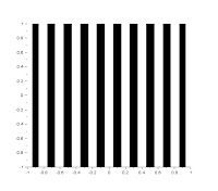
A = sin(X*width*%pi);

3. grating along the x-direction

For this part, I used the same code as in (2), but I changed the number of gray values to 2 (either black or white only). I also played with the number of slits by changing the variable width. The photos below show gratings with width equal to 500, 700 and 1000, respectively.

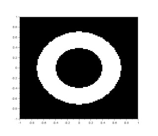
4. annulus

r = sqrt(X.^2 + Y.^2);
A(find(r<0.7&r>0.4)) = 1;

5. circular aperture with graded transparency (gaussian transparency)

sigma = 0.1;
r = sqrt(X.^2 + Y.^2);
A = exp(-r.^2/(2*sigma));

And now comes the fun part. I tried to create other patterns and really got the hang of it, and so I was able to create various patterns. The codes I used were just a combination of all the past I've used, and some were also new patterns.

Cross

A(find(abs(X)<=0.3|abs(Y)<=0.3))=1;

 Checkered

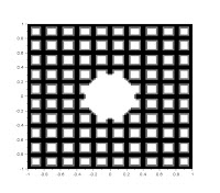
This has some variations: a plain checkerboard, checkerboard with circular center and checkerboard with square center.

B = ones(nx, ny);
width = 500;
a = sin(X*width*%pi);
b = sin(Y*width*%pi);
B(find(abs(a)<=0.6))=0;
B(find(abs(b)<=0.6))=0;
r = sqrt(X.^2 + Y.^2);
B(find(abs(X)<=0.5&abs(Y)<=0.5))=1; //for square center
B(find(r<0.3)) = 1; //for circular center

Half-circle and Quarter Circle

r = sqrt(X.^2 + Y.^2);
A(find(r<0.5&Y<0)) = 1; //for half-circle
A(find(r<0.5&Y<0&X>0)) = 1; //for quarter circle

I played around with quarter circles and the annulus and obtained a pattern slightly similar to the BMW logo.

A(find(r<0.5&((Y<0&X>0)|(Y>0&X<0)))) = 1;
A(find(r>0.7&r<0.9)) = 1;

Hourglass and Pinwheel

The first two is just a play with the angle Y./X. For the third photo, I just added a dark annular ring around the pinwheel.

r = sqrt(X.^2 + Y.^2);
angle = Y./X;
A(find(abs(angle)>=%pi))=1; //hourglass
A(find(abs(angle')>=%pi))=1; //pinwheel
A(find(r>0.7&r<0.9))=0; //add for dark annular ring

Beats

I also tried adding two sines with slightly close frequencies to produce a beat pattern. I did the same with two cosines and obtained a same pattern that was slightly shifted to the right. However, to see the pattern, I needed to increase the range to plot from (-1,1) to (-100,100).

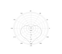
A = sin(X*10*%pi)+sin(X*10.3*%pi);
A = cos(X*10*%pi)+cos(X*10.3*%pi);

Lastly, I wanted to create a heart-shaped pattern, but I was not very successful. My idea is to plot a deltoid equation in polar coordinates and convert the plot into a 2d grayscale grid. I got the deltoid equation from a blog site on programming in Scilab. I was able to plot a heart like this:

t = linspace(-%pi,%pi,nx);
r = ((sin(t).*sqrt(abs(cos(t))))./(sin(t) + (7/5))) - 2*sin(t)+2;
polarplot(t,r);

Now, instead of using grayplot, I defined a polar grid C and used graypolarplot to render the plot in grayscale. However, the result I obtained is this:

C = round(t'*(1-r^2));
graypolarplot(t,r,C);

The heart was at the middle, but I could not remove the gradient outside of the heart shape. So far I've been searching for a way to fix this but I still can't.

Overall, I enjoyed this exercise because it was a great learning experience for me to learn and explore a new programming language. I'm pretty used to working and thinking in Python, and so it was refreshing (but a bit annoying at the start) to learn something new. I found several Scilab handbooks online which helped a lot, and some of my classmates helped as well.

Grade I give myself: 12/10. Aside from the minimum requirements, I was also able to explore and extend the activity to produce more patterns, earning the full bonus points. I would also like to acknowledge my classmates Justine Carpio, Norman Mascarinas and Wynn Improso for helping me translate my ideas into Scilab code. Lastly, I want to acknowledge a blog of a previous 186 student with alias dennisivan89 where I looked at his photos to check if I was indeed getting the right results, especially in the sinusoid pattern.